Article

Acceleration and Relocation of Abandonment in a Mediterranean Mountainous Landscape: Drivers, Consequences, and Management Implications

by
Diogenis A. Kiziridis
1,*,
Anna Mastrogianni
1,
Magdalini Pleniou
2,
Elpida Karadimou
1,
Spyros Tsiftsis
3,
Fotios Xystrakis
2 and
Ioannis Tsiripidis
1
1
Department of Botany, School of Biology, Aristotle University of Thessaloniki, 54124 Thessaloniki, Greece
2
Forest Research Institute, Hellenic Agricultural Organisation “Demeter”, 57006 Vassilika, Thessaloniki, Greece
3
Department of Forest and Natural Environment Sciences, International Hellenic University, 66132 Drama, Greece
*
Author to whom correspondence should be addressed.
Land 2022, 11(3), 406; https://doi.org/10.3390/land11030406
Submission received: 29 January 2022 / Revised: 1 March 2022 / Accepted: 7 March 2022 / Published: 10 March 2022

Abstract

:
Land abandonment in European mountains threatens habitats shaped for centuries by low-intensity agriculture and grazing. Hence, it is important to identify spatiotemporal patterns in rural abandonment, and relate them to biophysical and socioeconomic drivers. We pursued these goals in the theoretical context of transitions from traditional to productivist and then to post-productivist agriculture. We conducted a case study in a representative of southern Europe sub-mountainous marginal area that was once traditionally exploited (Pindus range, Epirus, Greece). Land cover was mapped from the outset of abandonment (years 1945, 1970, 1996 and 2015), and we subsequently calculated landscape metrics. An Intensity Analysis facilitated the comparison of rates of land cover change between time periods. By employing random forest modelling, we related socioeconomic, physiographic, geological and climatic predictors to land type occurrence and succession intensity. We found that farmland decreased from 30% to 3% during the 70 years of the study period, and that forest increased from 22% to 63%. The landscape’s heterogeneity, ecotone diversity, and spatial aggregation decreased. Abandonment and succession accelerated and relocated to lower elevation, especially during the latest time period, which was related to a second depopulation wave and livestock decrease. The remaining lowland farmlands were of productivist agriculture, and no widespread post-productivist regime was found. Thus, our study supports the view that policies, which have been mainly based on the linear transition of agricultural regimes in northern Europe, must take into account southern European mountains, where widespread abandonment can coexist with limited intensification and extensification.

1. Introduction

According to the European Red List of Habitats, habitats associated with farming activities are among the most threatened terrestrial habitat types [1]. In the mountainous regions of Europe in particular, the major threat to such habitats is the abandonment of low-intensity farming and traditional management practices, such as livestock grazing, mowing and burning [2]. Abandonment in these marginal areas commonly results in the succession of farmland and grassland by scrubland and, subsequently, by forests [3]. The biodiversity consequences of this afforestation have been disputed in the literature. On the one hand, afforestation increases the diversity of late-successional species, such as large mammals [4]. On the other hand, it threatens the mountainous grasslands, which are diverse communities hosting rare species [5]. For the Mediterranean Basin, which is a biodiversity hotspot facing intense abandonment, especially in the mountains, a meta-analysis has identified some factors that explain the contrasting consequences of abandonment [6]: diversity increases in the lowlands, especially in abandoned farmlands, but it decreases in uplands, especially in the abandoned grasslands of pastoral landscapes. For example, a study implemented adjacent to the present work’s study area in Greece found that afforestation after farmland abandonment was related to lower diversity and richness of bird species, especially of species associated with farmland and Mediterranean scrubland habitats [7].
Land abandonment has been attributed to different socioeconomic and biophysical conditions [4,8]. It is usually triggered by socioeconomic changes: farmers reduce or even cease land exploitation when it becomes unprofitable because of changes in agrarian policies or markets [9]. Socioeconomic changes can be imprinted on temporal trends in population and livestock densities, indicating migration, rural depopulation, and change of occupation [8]. Consequently, farmers are expected to abandon localities that incur higher exploitation costs earlier. The accessibility of a locality is a commonly related predictor of vulnerability to abandonment, assessed as distance to the road network or to the nearest settlement [10]. For the same economic reasons, biophysical conditions, such as physiography and soil fertility, also contribute to vulnerability to abandonment [8]. Besides any human intervention after abandonment, the consequent succession can have different rates in two areas abandoned simultaneously, depending on their proximity to roads and settlements, their species pools, physiography, geology, and climate [11].
In the same area, different rates of land cover change due to abandonment can also occur between time periods of different socioeconomic regimes. In Europe, the end of World War II (WWII), as well as of the Eastern Bloc, marked the initiation of abandonment [12,13]. Socio-political theory indicates two associated agricultural transitions after WWII. The first transition, from the traditional era of low-intensity farming to the productivist era of industrially driven agricultural intensification, was signalled by the objective of maximising food production via mechanisation after WWII [14]. This transition to productivist agriculture is commonly related to the loss or aggregation of small-sized, individually owned farms into large monocultural parcels in simplified landscapes [15]. As a consequence of the measures taken to this end by the European Union’s Common Agricultural Policy (CAP), less productive regions, such as in the uplands, lost the competition for funding against more productive regions in the lowlands [16]. The criticism of these effects of CAP resulted in a second transition, towards the post-productivist era, after the mid-1980s [14]. Part of the support was thereafter directed towards a more sustainable, diverse, and extensive agriculture in a countryside that itself became an object of consumption through the provisioning of tourism and other services. This transition can be evident by the reappearance of spatial differentiation in the landscape, where commercial agriculture coexists with forestry, multi-functional farming, and service-related land uses [15].
In Greece, similar to other Mediterranean countries, agriculture has not achieved a complete transition to the productivist era—as theory predicted for northern Europe—especially in rural areas of the uplands, where the abandonment of traditional farming is still ongoing [14]. This distinctive feature of Mediterranean mountainous landscapes supports the wider theoretical argument against the view of a spatially generalised and temporally linear regime shift from a traditional to a productivist and then to a post-productivist era [17]. Specifically, it has been argued that both intensive and extensive farming systems can instead coexist in a region [18]. This argument has been supported mainly on socio-political grounds, but more recent literature has contributed to the theoretical debate with empirical evidence from a land use and land cover perspective in Greece [19]. The latter authors found evidence of spatial differentiation instead of an overall transition to productivist agriculture. What is currently missing from this type of empirical study is a finer spatiotemporal resolution, together with a more quantitative analysis of factors besides elevation, to better capture the spatiotemporal characteristics of agricultural transitions in southern Europe.
To contribute to this theoretical debate, the present study aimed to test whether a linear agricultural transition or a coexistence of regimes has occurred, using empirical evidence from a case study in Greece. We mapped, in a fine spatiotemporal resolution, the land cover and related environmental conditions of a sub-mountainous area for a period of 70 years, starting from the end of WWII. The discussion of our results is presented in the context of the theoretical debate, and of the management implications for the maintenance and restoration of these historical but threatened landscapes.

2. Materials and Methods

2.1. Study Area: Biophysical and Socioeconomic Conditions

The study area comprised five circular sites 6 km in diameter with a total cover of 141.4 km2, located in the Pindus mountainous region in northwestern Greece (Figure 1). We chose this study area as a model system representative of the Mediterranean mountainous landscapes, because the wider region historically had extensive farmlands and grasslands traditionally exploited via low-intensity farming and transhumance until the 1940s, but subsequent land abandonment led to significant landscape changes [19].
The extent and location of the five study sites were chosen on the basis of criteria concerning vegetation diversity and identity because we conducted detailed vegetation sampling, aiming to investigate in depth, for another study, the consequences of land abandonment on vegetation and plant diversity attributes within the study sites. We preferred circular sites of sampling because they have the lowest perimeter-to-area ratio [20], and they therefore suffer less from edge effects [21]. We chose five such sites to maximise the total heterogeneity of the sampled gradients concerning environmental and vegetation diversity, as well as of land abandonment in recent and past trends. For the initial assessment of the latter factor of land abandonment, we consulted the results of a national land registry mapping project.
Based on the dominant woody taxa, the region belongs to the vegetation formation of thermophilous deciduous oaks [22]. The study area’s elevation ranges from 248 to 1203 m (Figure S1a of the Supplementary Materials). Most of the area is characterised by gentle slopes (0–10°), reaching a maximum of 55° (Figure S1b). The distribution of northness, i.e., the cosine of the slope’s aspect, is relatively symmetric between north- (+1) and south-facing (−1) aspects (Figure S1c). By contrast, the distribution of eastness, i.e., the sine of aspect, includes more east-facing aspects, i.e., more cover with eastness closer to +1, given that sites 3 and 5 occur on the east-northeast-facing side of a mountain mass (Figure 1 and Figure S1d). Regarding the parent rock, the study area has limestone, deposits, silicate, and flysch, in decreasing order of cover (Figure S1e).
The temperate climate of the study area is considered hot-summer Mediterranean, i.e., of “Csa” type according to the Köppen–Geiger classification system [23] (Figure S1f–x). Specifically, the mean temperature of the warmest month was above 22 °C, the mean temperature of the coldest month was commonly above −3 °C, and for at least three months it averaged above 18 °C. The precipitation was at least three times higher in the wettest month of winter than in the driest month of summer, and the driest month received less than 30 mm.
The study area experienced a population reduction during the study period (Figure S1y). The median of population density was more than halved during the last 70 years, i.e., from 27 inhabitants km−2 in 1945 to 12 inhabitants km−2 in 2015. Goats and, to a lesser extent, cattle and sheep, experienced a reduction in their densities as well (Figure S1z–ab). Finally, the expansion of settlements resulted in slightly reduced distances from any point on the map in time (Figure S1ad).

2.2. Data

We investigated the land cover and related predictor variables for the years 1945, 1970, 1996, and 2015 (Figure 2). The resulting maps of the land cover and the predictors were rasterised to square grids of 25 m resolution. Some predictors were fixed in time, i.e., the physiographic and geological, whereas others could take different values depending on the study year, i.e., the climatic and socioeconomic (Figure S1). All analyses were carried out in R [24].
As a base for the physiographic variables, we used the grid of the Digital Elevation Model over Europe at 25 m resolution [25]. We then generated 25 m rasters for the ground’s slope and aspect and, subsequently, for the northness and eastness, with the R package “raster” [26]. The map of the study area’s geological substrates was taken from [27].
For the climate, we considered the 19 bioclimatic variables of Worldclim. Each study year was represented by the average of a bioclimatic variable from the previous 10 years (study year included). The bioclimatic variables were calculated with the R package “dismo” [28]. We built the 25 m meteorological rasters for calculating the 19 bioclimatic variables by spatially interpolating coarser meteorological rasters with the R package “meteoland” [29,30]. The coarser meteorological rasters of 30 arc sec resolution were monthly time series of total precipitation, together with minimum and maximum temperature from the CHELSAcruts dataset [31].
Figure 2. Workflow of the present study. From lighter to darker fill, the boxes represent different types of input or output: raw data (white fill); raw data processing (light-shaded fill); processed data (dark-shaded fill); and analyses of processed data (darker-shaded fill with white letters).
Land 11 00406 g002
From the socioeconomic predictors, the population and livestock density in any district was the respective human and livestock population divided by the district’s area. For livestock, besides the cattle, sheep and goat densities, we additionally employed a combined “livestock density” variable, in small grazing livestock units km−2 (Figure S1ac). This variable was the sum of densities of the three livestock species, after multiplying the cattle density by the coefficient 6.66, to render the more demanding cattle equivalent to the less demanding sheep and goats [32]. The population and livestock densities held the same value in the 25 m raster cells inside a municipal district, with the five circular sites intersecting 35 districts (Figure 1). We obtained the data for the population and livestock from national censuses, retrieved from [33].

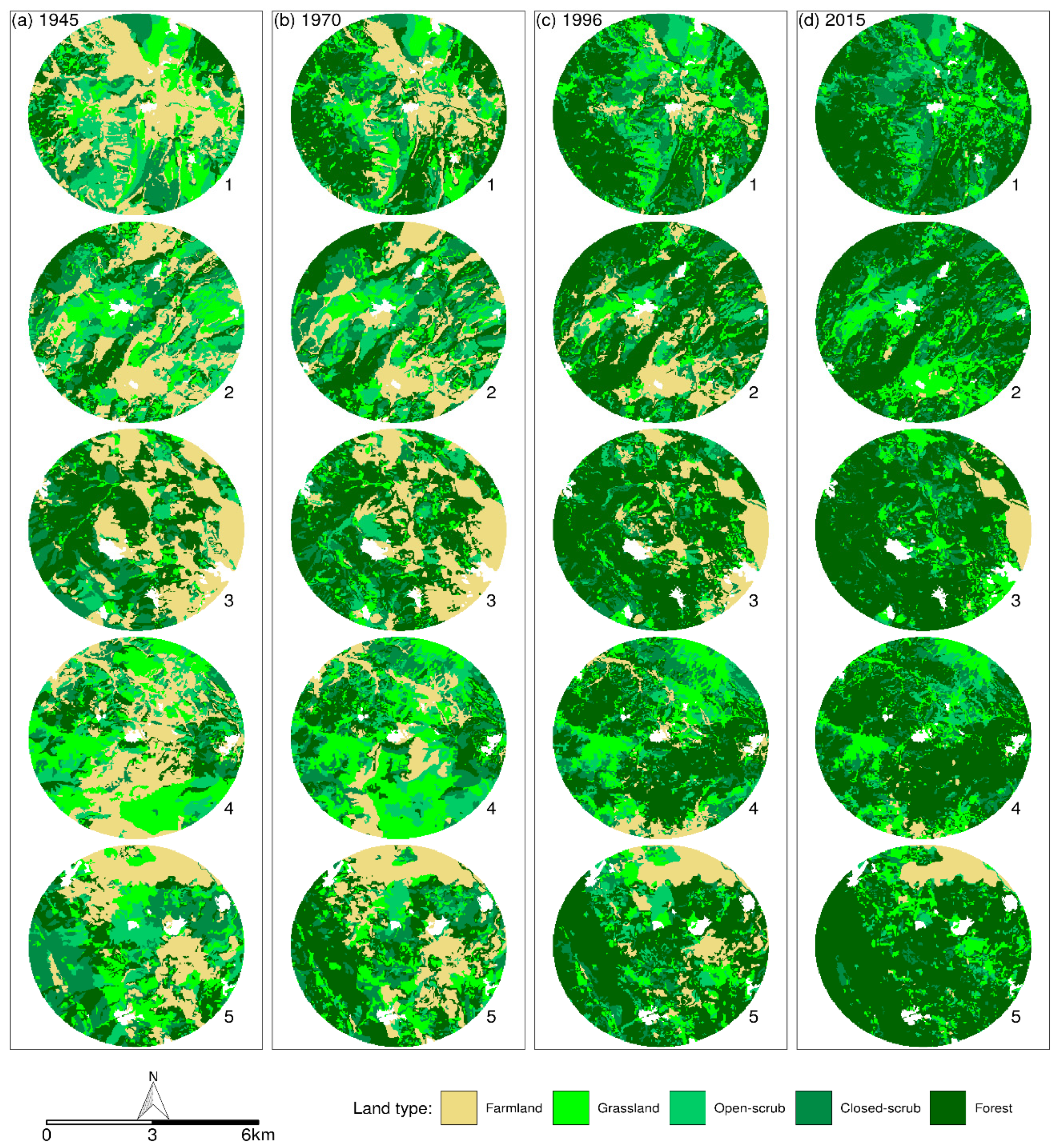
2.3. Mapping the Land Cover

We mapped land cover into five land types—namely farmland, grassland, open-scrub, closed-scrub, and forest—as vegetation formations indicative of secondary succession stages (results in Figure 3). We excluded settlements and water bodies from the analyses because they were irrelevant to the focal topic of the present study; hence, we worked with a remaining mapped total cover of 138.4 km2. We compiled a dataset of natural-colour orthophotos and large-scale aerial photographs for the four study years from three organisations: the Hellenic Cadastre, the Hellenic Military Geographical Service, and the Ministry of Rural Development and Food of the Hellenic Republic. Mapping was performed manually, by the visual interpretation of orthoimages, to achieve the adequate discrimination of the different land types, despite their spectral proximity across the non-homogeneous study area. This approach was selected since it allows well-trained human image interpreters, with personal experience and knowledge of the area, to clearly detect colour gradations and to integrate textural and contextual information at a small or medium scale [34,35].
A cover of 250 m2 was selected as the threshold of the minimum cover for vectorisation. Vectorisation of the land type boundaries was followed by the rasterisation of the maps to a 25 m resolution. Visual interpretation was supported by field sampling, and by various ancillary data (CORINE and “Google Earth” maps). The vegetation cover thresholds used for the interpretation of grassland, open- and closed-scrub, and forests, were the following: grassland, cover of scrub-tree species less than 10%; open-scrub, cover of scrub-tree species in the range of 10–40%; closed-scrub, cover of scrub-tree species in the range of 40–70%; and forest, cover of scrub-tree species greater than 70%. The same thresholds have been used in the past for a national forest mapping project [27].
The 1970 aerial photographs required orthorectification. We implemented photogrammetric procedures to compensate for geometric errors induced by different sources, including image distortions created by terrain variations [36]. The aerial photographs were primarily processed with the already orthorectified images from 2015 as reference data, and secondarily with images from the other years. To achieve the best possible geometric matching of the images, we identified well-distributed ground-control points by using visible landmarks on aerial orthophotos and on uncorrected aerial images. For the orthorectification, we employed a Digital Elevation Model with a 5 m resolution, provided by the Hellenic Cadastre. We preferred nearest-neighbour resampling to avoid any smoothing effects. Checks of the geometric model indicated an acceptable level of error. To ensure spatial compatibility, we adopted the projection of the Greek Geodetic Reference System throughout (EGSA 87).

2.4. Quantifying Spatial Aspects of the Landscape over Time

We calculated four spatial metrics at the landscape level for each study site and year (results in Figure 4): relative marginal entropy, largest patch index, interspersion and juxtaposition index, and relative mutual information [37,38]. We calculated the four landscape metrics with the R package “landscapemetrics” [39]. These metrics were max-normalised to take a maximum value of one, whereas their minimum values could not be less than zero. Apart from the comparability between sites and study years due to this normalisation, we selected these metrics to elucidate different aspects of the landscape [38].
Specifically, the following four aspects of the landscape were quantified with the four corresponding metrics (Table 1):
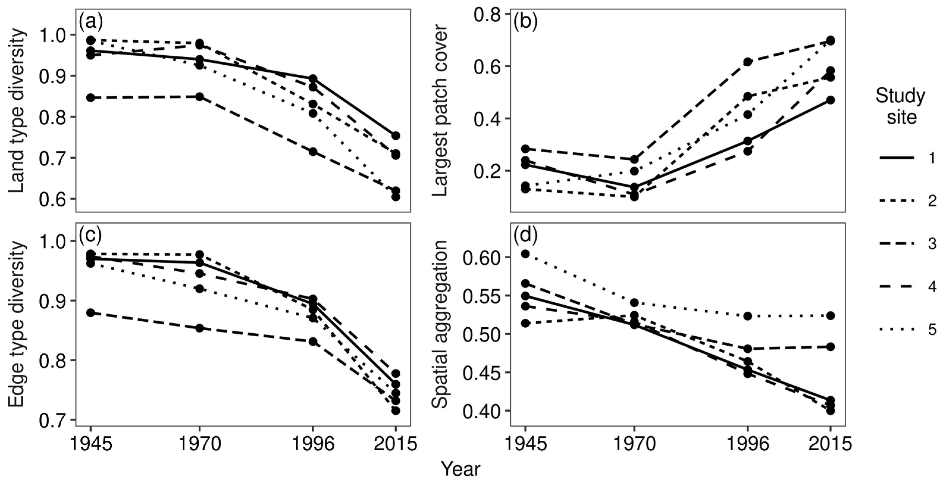
  • Land type diversity, with relative marginal entropy. Relative entropy quantifies the diversity of land types relative to the maximum value. It attains its maximum of one when relative cover is evenly distributed among the land types, whereas the minimum of zero is taken when one land type covers everything.
  • Largest patch cover, with the largest patch index. This index gives the area of the largest patch divided by the total area. Its maximum is one when the largest patch is the landscape itself, and its minimum approaches zero in larger landscapes that are more spatially disaggregated and rich in land types.
  • Edge type diversity, with the interspersion and juxtaposition index. This index measures the diversity of edge types relative to its maximum value. It is maximally one when relative edge length is evenly distributed among different types of edge between any possible pair of land types. It is minimally zero when there is only a single edge type, i.e., between two specific land types.
  • Spatial aggregation, with the relative mutual information. It quantifies the information that a focal raster cell’s land type provides for the prediction of an adjacent cell’s land type, relative to its maximum value. Its maximum of one is attained when the landscape is of one land type, and its minimum approaches zero when the land type prediction of a neighbouring cell can be, at best, random.
Table 1. Landscape aspects with the corresponding metrics and their equations.
AspectMetricEquation 1Ref.
Land type
diversity
Relative
marginal entropy
H = i = 1 L ( c i log 2 c i ) / log 2 L [37]
Largest
patch cover
Largest Patch
Index
L P I = max 1 n N ( p n ) [36]
Edge type
diversity
Interspersion and
Juxtaposition Index
I J I = i = 1 L j = i + 1 L ( e i , j ln e i j ) / ln L ( L 1 ) 2 [36]
Spatial
aggregation
Relative mutual
information
U = i = 1 L j = 1 L ( c i j log 2 c i j c i c j ) / H [37]
1 Notation: L (number of land types); c i (relative cover of pixels with land type i); N (number of patches); p n (relative cover of patch n); e i j (relative length of edge between land types i and j); and c i j (relative cover of adjacent pixels with land types i and j).

2.5. Analysing the Rates of Land Cover Change

We applied an Intensity Analysis to pairs of land cover maps from consecutive study years to identify rates of land cover change at three levels of increasing resolution (equations in Table 2; results in Figure 5 and Figure 6): overall change, land type change, and a specific land type transition [40]. At any level of change, the Intensity Analysis can express the rates in absolute or relative terms. At the level of overall change, we can obtain the absolute or relative cover of the landscape changing annually during a time period. At the level of land type change, we can calculate the absolute gain (loss), i.e., the cover that a land type gains (loses) annually during a time period; the rate of relative gain (loss) expresses the percentage of the land type’s final (initial) cover that is gained (lost) annually. At the level of transition from land type k to land type l, the absolute transition rate is the cover of land type k that is annually converted to land type l during a given time period, whereas the relative transition rate expresses the percentage of land type k converted annually to land type l during this period. We carried out the Intensity Analysis with the R package “OpenLand” [41].
The relative change rates at the level of land type can be compared with the rate of landscape relative change to identify land types that change faster or slower than average. Stationarity can be inferred when a land type consistently gains or loses faster or slower than the rate of the landscape’s relative change throughout all time periods [40]. Additionally, such comparisons between annual rates can identify specific trends in intensity of change across time periods, i.e., whether land type change accelerates, decelerates, or remains stable between periods. Similarly, at the level of a specific transition, a land type’s relative transition rate can be compared to the rate of the land type’s overall relative change to test whether the specific transition is faster or slower than the land type’s mean relative change. Again, these comparisons can be used to test for stationarity and to identify trends in the intensity of land cover change, i.e., whether a specific transition accelerates, decelerates, or remains stable between time periods. Finally, the annual form of the rates permits the comparison of land cover change between time periods of different lengths, as in our case study.
Table 2. Level (Lv.) of land cover change and the equations 1 for the Intensity Analysis [39]. For each level, rates of mean relative gain and loss are provided below the respective rates of relative change.
Lv.Absolute GainAbsolute LossRelative GainRelative Loss
Overall l = 1 L [ k = 1 L ( C t k l ) C t l l ] P t l = 1 L [ k = 1 L ( C t k l ) C t l l ] P t 100 l = 1 L [ k = 1 L ( C t k l ) C t l l ] P t C 100 l = 1 L [ k = 1 L ( C t k l ) C t l l ] P t C
Mean relative gain and loss: 100 t = 1 T { l = 1 L [ k = 1 L ( C t k l ) C t l l ] } P C 100 t = 1 T { l = 1 L [ k = 1 L ( C t k l ) C t l l ] } P C
Land type k = 1 L ( C t k l ) C t l l P t l = 1 L ( C t k l ) C t k k P t 100 [ k = 1 L ( C t k l ) C t l l ] P t k = 1 L C t k l 100 [ l = 1 L ( C t k l ) C t k k ] P t l = 1 L C t k l
Mean relative gain and loss: 100 l = 1 L [ k = 1 L ( C t k l ) C t l l ] P t C 100 l = 1 L [ k = 1 L ( C t k l ) C t l l ] P t C
Transition C t k l P t C t l k P t 100 C t k l P t m = 1 L C t k m 100 C t l k P t m = 1 L C t m k
Mean relative gain and loss: 100 [ k = 1 L ( C t k l ) C t l l ] / P t m = 1 L [ k = 1 L ( C t k m ) C t l m ] 100 [ k = 1 L ( C t l k ) C t l l ] / P t m = 1 L [ l = 1 L ( C t m k ) C t m l ]
1 Notation: t (index of time period); P t (duration of time period t, in years); C t k l (cover of study area that transitioned from land type k to land type l at the time period t, in km2); C (total cover of the study area); P (total duration of the study period); and T (the number of time periods).
To relate any changes in the rates between time periods with socioeconomic changes, we statistically compared the annual percentage change in the population and livestock of the 35 municipal districts across the time periods (results in Figure 7). Due to outliers, non-normality, and unequal variances between time periods, we could not use an ANOVA for repeated measures of each municipal district in time, and we instead used a non-parametric, Friedman-based post hoc test returning exact p-values [42]. By assuming that any time-lagged socioeconomic effect would be negligible because the three time periods were relatively long, we focused on the relation between the socioeconomic changes in a period with the rates of relative change in land cover for the same period.

2.6. Modelling the Occurrence of the Land Types

We related land type occurrence to biophysical and socioeconomic variables with a random forest multiclass classification model (results in Figure 8). We employed random forest models in this study because they have few parameters to tune, they are not restricted by assumptions about the distribution of variables, and can handle non-linear relationships, unlike linear models [43]. Additionally, in a spatial context, a random forest does not require the complex modelling of semivariograms with their related statistical assumptions [44]. Our classification model predicted the probability of each land type—averaged among individual classification trees—on each raster cell given the cell’s predictor conditions. From the pool of predictor variables (Figure S1), we selected a subset on the basis of lower inter-correlations (Spearman correlation coefficient not greater than 0.5), but also higher interpretability of model results (Figure S2). Specifically, we employed the elevation, slope, northness, eastness, presence of silicate and flysch parent rock, temperature and precipitation seasonality, population and livestock density, and distance to the nearest settlement. We additionally employed the longitude and latitude as extra predictors to capture spatial autocorrelations [45].
The random forest model was parameterised and fitted on a balanced random subset of the whole dataset, i.e., a training dataset of n observations. Specifically, in any combination of land type, study site, and year, the minimum number of observations was 92. Hence, we randomly selected 92 observations from each combination of land type, study site, and year, leading to a training dataset with a total of n = 92 × 5 × 5 × 4 = 9200 observations of land type cover and corresponding predictor values. With the R package “caret” [46], model hyperparameters were fine-tuned by 10-fold cross-validation. We tried the different combinations between split rule (“gini” or “extratrees”) and number of randomly selected predictors to consider at each split (two, half or all of the variables), selecting the combination that maximised the classification performance in terms of the metrics “Accuracy” and “Kappa”. The hyperparameter for the minimum number of observations in the terminal nodes of individual trees was fixed at equal to one. Finally, the hyperparameter for the number of trees was fixed at equal to the computationally feasible count of 1000, since it has been shown that it is not necessary to fine-tune this hyperparameter [47].

2.7. Modelling the Intensity of Farmland and Grassland Succession

We employed two random forest regression models to predict the intensity of farmland and grassland succession at the raster cells that were, respectively, farmland and grassland in 1945, and that were persisting or moving only forward in the progressive successional pathway (results in Figure 9). Specifically, succession was assumed to progress according to the following pathway: farmland → grassland → open-scrub → closed-scrub → forest. Succession intensity is a metric we invented to quantify how quickly and how much a cell progresses in succession through time. It is the normalised area under the curve of a cell’s successional trajectory (Figure S3). The normalisation is based on the maximum area under the curve, which was achievable in this study when a 1945 farmland or grassland pixel turned to forest in 1970. Succession intensity hence took its minimum value of zero when a cell that was farmland or grassland in 1945 persisted as such until the last study year, 2015. Thus, our metric could capture trajectories in the range from complete farmland and grassland persistence during the 70 years, to afforestation in just 25 years (from 1945 to 1970). Notably, although studying retrogressive succession would have been of equal interest, we focused on progressive succession because a very low proportion of vegetation transitioned retrogressively, and because the present study was primarily concerned with land abandonment.
The succession intensity metric encapsulated a temporal process in a single value (Figure S3). Consequently, the temporal trends of the time-varying variables from our set of selected predictors were also required to be summarised in a single value. For the population and livestock densities, and the temperature and precipitation seasonalities, we employed the slopes of linear models fitted on their time series. For comparability, the time series were divided by their 1945 value before fitting a linear model; they therefore expressed the annual rate of change relative to the study period’s initial value. For the settlement proximity, we kept the mean of the study years, since it did not change considerably over time. The variables that did not need to be processed were those that were fixed in time: elevation, slope, northness, eastness, presence of silicate parent rock, presence of flysch parent rock, plus longitude and latitude.
Again, we used a training dataset of n observations for the parameterisation and fitting of the farmland and grassland succession models. For the farmland succession model, we randomly selected 2000 cells that were farmland in 1945, and that persisted or moved only forward in the expected successional pathway from each of the five study sites, leading to a training dataset with a total of n = 2000 × 5 = 10,000 observations of farmland intensity of succession and corresponding predictor values. Similarly, for the grassland succession model, we randomly selected 1549 cells that were grassland in 1945 from each of the five study sites, and that persisted or moved only forward in the expected successional pathway (the study site with the minimum number of appropriate observations had 1549 such pixels), leading to a training dataset with a total of n = 1549 × 5 = 7745 observations. The two models were parameterised and fitted similarly to the random forest model of land type occurrence. However, since these two models were of the regression type, they featured the following differences from the random forest classification model of land type occurrence: the tested split rules were “variance” and “extratrees”; the performance metrics were the root-mean-square error, the R-squared, and the mean absolute error; and the minimum number of observations in the terminal nodes of individual trees was fixed at equal to five.
Figure 3. Land cover maps of the five sites, for the following years: (a) 1945; (b) 1970; (c) 1996; and (d) 2015. The sites are numbered as in Figure 1.
Land 11 00406 g003

2.8. Displaying the Results of the Random Forest Models

A relation between a response variable (probability of land type, or succession intensity) versus a predictor variable was presented by the predictor’s mean of individual marginal effects [48]. An individual marginal effect of a predictor’s specific value was the predicted value of the response variable when the rest of the predictors took one of their n observed combinations of values from the training dataset. Subsequently, for the range of the focal predictor’s observed values, a so-called partial dependence plot displayed the LOESS curve of the mean among the n individual marginal effect curves (Figure 8 and Figure 9). We additionally inspected a random sample of the n individual curves, validating the representativeness of the mean curve (Figures S4–S6). Only the predictor variables with the most representative means were chosen to be shown in the Results. The R package “pdp” produced the data for the partial dependence plots [49].

3. Results

3.1. History of Land Cover, Landscape Aspects, and Land Cover Change

Land abandonment and succession were visually apparent in the maps of the study sites over time (Figure 3). The once extensive farmland of 1945 (Figure 3a) was mainly limited to only two relatively large patches at sites 3 and 5 in the last year, 2015 (Figure 3d). Similarly, only a few large patches of grassland persisted after 1945, such as the two grasslands at the north–northeast and west of site 4. The landscape metrics captured the ongoing abandonment and afforestation, such as in the reduction in the diversity of land types in the more recent years (Figure 4a). Additionally, while the largest patches in the earlier years were farmlands and grasslands covering around 15–30% of a site, forest occupied the largest patches of the later years, with a greater relative cover of around 45–70% of a site (Figure 4b). The withdrawal of farmland and grassland, and the expansion of forest, also led to poorer diversity of ecotones between different land types (Figure 4c), apparently with the domination of forest-neighbouring edges (Figure 3). Despite this overall forest domination, the landscape became more fragmented at a relatively slow rate (Figure 4d), often due to the replacement of large farmland and grassland patches by smaller grassland and scrubland remnants in the expanding forest matrix (Figure 3).
Figure 4. Landscape aspects of the sites over the study period. The four metrics for the four corresponding aspects of the landscape were the following: (a) relative marginal entropy; (b) largest patch index; (c) interspersion and juxtaposition index; and (d) relative mutual information. These landscape metrics reached a maximum value of one upon division by their maximum possible value. The sites are numbered as in Figure 1.
Land 11 00406 g004
Apart from its spatial signature, abandonment was also evident in the 89.4% relative decrease in farmland cover, from 30.2% of the study area, which was the largest share among land types in 1945, to 3.2%, which was the smallest in 2015 (Figure 5a). By contrast, the consequent afforestation resulted in a 188.5% relative increase in forest cover, from 21.7% to 62.6% of the study area during the 70 years. Grassland, open- and closed-scrub kept a relatively stable cover over time. Nevertheless, these intermediate successional stages participated dynamically in the conversion of farmland to forest (flows in Figure 5a). The vast proportion of cover transitioned in the direction of progressive succession; the smaller transitions in the direction of retrogressive succession decreased even further over time. Focusing on the fate of the 1945 farmland and grassland, a wide range of progressive successional pathways unravelled, from their 70-year persistence until 2015, to their afforestation after just 25 years (Figure 5b,c). Notably, farmland accelerated its transition to other land types over time, especially to grassland (Figure 5b).
Figure 5. Land type cover and transitions over the whole study period. Bars indicate the cover of each land type in the study years, and flows between years depict the following: all land type transitions (a); the progressive successional pathways of the pixels that were farmland in 1945 (b); and the progressive successional pathways of the pixels that were grassland in 1945 (c).
Land 11 00406 g005
The Intensity Analysis confirmed quantitatively this last observation of accelerated farmland loss in particular, and of the acceleration of succession in general. Although the absolute cover lost by farmland was similar between the time periods (Figure 6a), the relative loss rate almost doubled, exceeding the rate of mean landscape change during the last two time periods (beyond the negative dashed lines in Figure 6b). In fact, this relative loss of farmland was the only type of land cover change that significantly exhibited non-stationarity, i.e., by exceeding the mean relative loss of the landscape from the first to the second and third periods (Figure 6b). Additionally, the farmland-to-grassland rate of transition was the only one among the rates of farmland loss that increased during the last time period both in absolute (Figure 6c) and in relative terms (Figure 6d). Grassland, open- and closed-scrub also increased their rates of relative loss and gain during the last time period (Figure 6b,d), despite the stability in their rates of absolute change (Figure 6a,c).
Figure 6. Intensity of land type change at two levels of resolution. At the land type level, the negative values are annual rates of land type loss in absolute terms (a), and relative to the land type’s cover at the start of the period (b); the positive values are for a land type’s absolute annual gain (a), and in relation to its cover at the end of the period (b). At the land type transition level, the negative values are annual rates of absolute (c) and relative (d) transition to forest from the other land types, whereas the positive values are for farmland becoming other land types in absolute (c) and relative terms (d). The dashed lines indicate rates of mean change according to the previous resolution level of the landscape change for panel (b), and of the land type change for panel (d).
Land 11 00406 g006
These increased rates of abandonment and succession during the last time period corresponded to significantly higher rates of population and livestock decrease in the municipal districts during that period (Figure 7).
Figure 7. Distributions of annual percentage change in population (a), and livestock (b), in the 35 municipal districts in the three time periods. Each violin plot displays the mirrored density distribution of the 35 values. The letters above the distributions indicate the grouping based on Friedman-type post hoc tests of equality between the time periods (repeated measures of each district in time).
Land 11 00406 g007

3.2. Conditions Related to the Occurrence of the Land Types

According to the classification model, the probability of finding farmland was higher at slopes lower than around 20°, and at elevations lower than around 750 m (Figure 8a,b). Farmland was not associated strongly with northness (Figure 8c). Socioeconomically, farmland was more frequent at higher population and livestock densities, which were more commonly documented in the earlier years (Figure 8d,e).
Figure 8. Mean marginal effects of the top five predictor variables most strongly related to land type occurrence: (a) slope; (b) elevation; (c) northness; (d) population density; and (e) livestock density. The vertical marks under the horizontal line indicate each predictor’s n observed values in the training dataset. In case of a predictor taking different values in different study years, the vertical marks are arranged in four rows, each row for a year, with the values of 1945 in the top row followed by 1970, 1996, and 2015, from top to bottom row.
Land 11 00406 g008
Grassland, like farmland, was more frequent in localities with slopes of less than 20°, but at elevations greater, not smaller, than 750 m (Figure 8a,b). Similarly to farmland, grassland was more commonly found with higher populations and livestock densities (Figure 8d,e). From the rest of the land types, forest showed the greatest influence according to the studied biophysical predictors, occurring more often in localities with greater slopes (with the occurrence increasing faster until slopes of approximately 20°), and more north-facing aspects (with the turning point at the west- and east-facing aspects of zero northness) (Figure 8a,c). Socioeconomically, forest was steadily more frequent at lower population densities, and for livestock densities of less than approximately 300 small livestock grazing units per square kilometre (Figure 8d,e).
The model exhibited a moderate land-type classification accuracy of 0.5, with a Kappa of 0.37.

3.3. Conditions Related to the Intensity of Farmland and Grassland Succession

The farmland in 1945 was abandoned sooner, and experienced more intense succession, at higher elevations, until approximately 750 m, higher slopes, up to approximately 20°, and more north-facing aspects (Figure 9a–c). The studied socioeconomic conditions did not appear to have a strong relation with the intensity of the farmland’s succession (Figure 9d,e). The model fit had a mean absolute error of 0.15 (in the 0–1 value range of the succession intensity metric), explaining 52% of the variance.
Figure 9. Mean marginal effects of the top five predictor variables most strongly related to intensity of farmland and grassland succession: (a) slope; (b) elevation; (c) northness; (d) population density; and (e) livestock density. For comparability, the curves are centred to the mean prediction at the left-most, minimum value of each predictor. The vertical marks under the horizontal line indicate each predictor’s n observed values in the training dataset of the model for farmland (top row of marks) and of the model for grassland (bottom row).
Land 11 00406 g009
For the grassland of 1945, progressive succession was, similarly to the farmland, more intense at higher slopes until approximately 20°, and with more north-facing aspects, but at elevations that were lower than 750 m (Figure 9a–c). Unlike farmland, the studied socioeconomic conditions appeared to have a strong relation with grassland’s intensity of succession. Regarding humans, the succession of the 1945 grassland was steadily more intense in municipal districts with an annual population decrease of higher than approximately −0.8% (Figure 9d). Regarding livestock, this grassland’s succession was more intense only in municipal districts that exhibited an overall livestock decrease, becoming steadily more intense at higher annual decreases in livestock (Figure 9e). The model fit had a mean absolute error of 0.16 (in the 0–1 value range of the succession intensity metric), explaining 57% of the variance.
Focusing on elevation, which was the strongest predictor of both farmland and grassland succession intensity, we can confirm that the abandoned and encroached farmland’s mean elevation was above the land type’s mean in all the time periods, while the encroached grassland’s mean elevation was lower than the overall grassland’s mean only during the last time period (Figure 10). Nevertheless, farmland abandonment kept relocating to lower elevations. Grassland followed the spatial shift of farmland’s abandonment with one period’s time-lag, by becoming encroached at higher elevation during the second period (1970–1996), where farmland was abandoned in the first period (1945–1970), and then in lower elevations, following farmland’s altitudinal descent of abandonment. Due to the relocation of encroachment to lower elevation, the mean elevation of both land types reached its lowest value in the last year, 2015 (vertical dashed lines in Figure 10).

4. Discussion

Our case study on the 70-year history of a Mediterranean mountainous landscape did not support the theoretical view of a spatially widespread transition from the traditional to the productivist era in the 1940s, followed by another transition towards post-productivism in the 1980s. Specifically, the transition in the form of farmland abandonment was intense, and even accelerated, and it was accompanied by the relocation of farmland to lower elevations. The consequent afforestation reduced the landscape’s heterogeneity, decreasing the diversity of land cover types and ecotones. Thus, our results supported instead the theoretical counterview of spatially differentiated countryside, where abandoned uplands coexist with agriculturally intensified lowlands.

4.1. History of Land Cover, Landscape Aspects, and Land Cover Change

The magnitude of abandonment and succession in our study area was in agreement with other studies in the region [19], in other mountainous regions of Greece [13], and in other Mediterranean regions [50]. For example, our 89.4% relative decrease in farmland was of the same magnitude as the more than 90% withdrawal cited for the Spanish Pyrenees and the Iberian Range [51]. Moreover, the observed landscape homogenisation due to forest domination, together with the persistence of smaller, but more numerous, grassland and scrubland remnants, is a common spatial pattern appearing in different abandoned mountainous regions [52]. Thus, the size and the spatial characteristics of abandonment and afforestation in our study area constitute the first line of evidence for the absence of a widespread transition to a productivist regime. In support of the view of [17], our study area illustrates that the theoretical notion of a widespread intensification of existing farmland, which has been confirmed in northern Europe, is not applicable to the marginalised mountains of southern Europe.
Although our results agree with the literature on the magnitude and spatial characteristics of landscape change, the rates of change showing the acceleration of abandonment and succession have rarely been reported [53]. Succession rates after abandonment are expected to decrease with time as more vulnerable localities become scarcer [50]. In our case, farmland was abandoned more than twice as quickly when it covered 12.2% of the landscape, in 1996, than when it covered 30.2%, in 1945; and the relative change rates of grassland, open- and closed-scrub substantially increased. Nevertheless, we expect that the accelerating trend in the abandonment and consequent succession will inevitably pass the turning point towards deceleration, as has been observed in nearby regions of Albania and Romania [54].

4.2. Conditions Related to The Occurrence of the Land Types, and the Succession Intensity

A main reason for expecting the deceleration of abandonment in our study area is that much of the remaining farmland has transitioned to a productivist regime. These farmland localities, especially the two large farmland patches in sites 3 and 5, have lower elevation and gentler slopes, which correlate with the presence of alluvial deposits, indicating more productive fields. Another characteristic that suggests a productivist regime in these two farmland patches is the presence of irrigation infrastructure. Irrigation infrastructure in the region was developed in the 1950s–1980s, with the aim of facilitating the transition to productivist agriculture [19]. As the latter authors note, however, Greek state programs contributed to the agricultural modernisation of only the productive plains in the lowlands, such as of the two patches. Thus, our study area aligns with the theoretically and empirically supported view of upland abandonment coexisting with lowland intensification in southern European mountains [18,19]. Even within the same municipality, we observed the abandonment of marginal land in the uplands and the agricultural intensification of lowland fields. This is clearly depicted in our results, and it has also been demonstrated for other Mediterranean mountainous areas [13,19,55].
Although our models did not show any strong relations between population or livestock change and farmland abandonment at the pixel level, the acceleration of farmland loss during the third time period corresponded to a significantly higher decrease in population and livestock densities at the municipality level. Depopulation in the area was indicated by two time periods of mainly negative population change, separated by an intermediate period of average stasis. In the 1945–1970 time period, depopulation was intense after WWII due to urbanisation, and because the region was one of the harshest theatres of the subsequent Greek Civil War [19]. In the 1970–1996 time period, the mixed and dispersed socioeconomic changes in the municipalities can be attributed to the new agricultural policies and measures by Greek governments and the European Union, which partially mitigated depopulation, but also forced the occupational reorganisation of the persisting population [56]. In the 1996–2015 time period, the high increase in abandonment and succession in the area, and the declines in population and livestock, can be said to be due to both the late-arriving and mistargeted measures for low-intensity farming of the previous period [19] and to the financial crisis during the period itself [57].
For grassland, the observed temporal stability of its relative cover in our study area was not accompanied by spatial stability, i.e., historical grasslands were commonly lost from the lowlands, appearing initially in place of the more intensively abandoned farmlands of the uplands and, later, in the lowlands, as they followed the altitudinal descent of farmland abandonment. Nevertheless, the historical grasslands of 1945 did persist at higher elevation in our study area, a phenomenon recently observed in other regions as well [58]. In the absence of relevant data, we can attribute this “mountain effect” to the traditional land use of vertical transhumance in the region [19], or to the arrest of succession by biophysical conditions, such as poorer soils [59].
Furthermore, grassland’s intensity of succession was more positively related than farmland to northness, as well as to human and livestock decreases. Increased northness can be linked to increased moisture availability, a condition that is often associated with increased rates of vegetation development in undisturbed grasslands [55]. Regarding the relation of population and livestock decreases with succession intensity, grassland persistence appeared to be a better indicator of occupation in the primary sector. Farmland persistence, by contrast, was not necessarily related to lower depopulation because less-depopulated municipalities with higher farmland abandonment in the region managed to keep more residents by redirecting their interest to tourism, trade in imported products, and other services [19]. Although the core of touristic development is mainly observed in adjacent municipalities, outside our study area, studied municipalities, such as Kalpaki, gradually developed into locally central towns, slowly transforming the surrounding countryside from one of agricultural production to one of “consumption of the countryside” [17]. This appearance of post-productivist signs in some localities can be added to the picture of coexisting regimes in our study area. Nevertheless, such signs are not equivalent to a full transition, as we discuss below.

4.3. Management Implications

Despite the signs of the development of a post-productivist regime in the study area, e.g., the increasing demand for ecosystem services, such as tourism, there was not a widespread reversal towards agricultural extensification and landscape diversification, which are characteristic of post-productivist regimes [14]. A similar pattern has been documented for a nearby area, where a full transition to a post-productivist regime was not found, even at a small scale [19]. On the contrary, abandonment and afforestation continued with the same and even higher rates in later years. Additionally, for the abandoned rural areas of Greece, only a few plans or policies have been implemented for reversing the state of threatened habitats, such as the LIFE+ JunEx project for the restoration of Grecian juniper silvopastoral woodlands [60]. Given the threats that such valuable ecosystems face, there is a great need to implement management plans for the numerous semi-natural landscapes of this mountainous country [61].
The magnitude and spatial characteristics of land cover change can inform such management plans to take into account both the amount of forest to be cleared but also the spatial distribution of targeted localities, as has been demonstrated in the Iberian range [51]. In our study area, for instance, deforestation could aim to reconnect grassland and scrubland remnants, for enriching ecotone diversity and consequently biodiversity [51], for fragmenting the forest to limit wildfire spread [62], and for enhancing the recruitment of grassland plant species which are commonly poor dispersers [63]. Another proposed approach is funding support for extensive stockbreeding, which can encourage residency in the region, engage residents with alternative sources of income, such as traditional cheese-making, ultimately contributing to the restoration and maintenance of the historical landscape [51]. Measures for reorganising historically multifunctional landscapes may be discouraged by the recent acceleration of abandonment in our study area. Nevertheless, the alternative of rewilding can incur greater costs by increasing wildfire risk, reducing lowland streamflow, and accelerating the vicious cycle of rewilding–depopulation [51].
In general, the regional planning and management of such semi-natural landscapes can be improved by a better understanding of the historical trajectories of agricultural regime shifts and their relation to biophysical and socioeconomic conditions [19]. At the same time, agricultural policies are essentially tools of rural management, and they can be considered significant factors of change in rural landscapes. Unfortunately, if planning is not based on such an understanding of local conditions, change in rural landscapes might follow trajectories that are different from those intended by their associated agrarian reforms. As an example from the 1950s–1980s period, which is applicable to our study region, Greek governments implemented agrarian policies, and development projects, such as irrigation, following the development of the productivist view of agriculture in western and northern Europe at that time [56]. Nevertheless, the different topographical characteristics of the numerous hilly and mountainous Greek regions limited the applicability of these policies, leaving such regions to follow an abandonment trajectory instead. As another example from the next period, of the 1980s–2010s, the post-productivist view of current policies [64] has not always and everywhere contributed to a significant transition towards an associated extensification and diversification of the primary and tertiary sector, as shown in our study of a mountainous Mediterranean region. It is therefore important to update the theory and policy of agricultural change with information from southern Europe, allowing them to be used more effectively as tools of regional planning and management.

4.4. Study Limitations and Future Directions

The inability to relate with greater certainty the persistence of historical grasslands in the uplands to other underlying conditions reveals a limitation of our study: the lack of data on other drivers and consequences of abandonment. Regarding these drivers, predictors strongly related to land cover change, e.g., parent rock, were easily obtained but might constitute surrogates of more proximate and informative drivers that are more expensive to obtain, such as soil fertility [10]. Another example is population change, which did not prove a good surrogate for occupation. Other socioeconomic variables related to employment were not available at the municipality level, nor for the time span of our study. Regarding the consequences of abandonment, our exclusive use of land-cover-type response data limited our interpretation. Complementary data on species distribution could help to distinguish plant communities in different land cover types and, hence, relate abandonment and succession to more specific conditions, a work that is in progress for our study area.
Given the variety of identified drivers and of their effects, an extension of our study with implications for planning would consider the optimised selection of localities for management. This maximisation of the environmental benefits would at the same time incur lower costs compared to a spatially uniform or random selection of localities [65]. For example, an optimisation algorithm or mathematical programming model would aim to find which localities are best to restore for a limited restoration budget, based on our identified drivers. Nevertheless, more drivers must be taken into account for planning, such as the population’s age structure, trends in agricultural product prices versus input prices, and local education and health infrastructure. All these must be coupled by field sociological studies in order to result in a concrete management plan.
The aforementioned field of sociological studies bring forth another dimension of our study: the spatial and temporal resolution of some studied variables and general aspects. Regarding the temporal resolution, the advantage of the present work over other similar studies of land cover change over a long time span is the use of three time periods, given that most studies that include data from the 1940s commonly present one or two time periods [66]. Nevertheless, future work could focus on further increasing the temporal resolution by adding maps of land cover and related variables between our studied years, to shed more light, e.g., on the relation between the recent acceleration of abandonment and the underlying socioeconomic changes during the time periods. Regarding the spatial resolution, and especially given the high variability of the drivers due to the spatial heterogeneity of the mountainous environment, field sociological studies could gather data at a spatial level lower than the current level of municipality, e.g., at the household level. This specialised information, of higher spatial resolution, would be valuable in the determination of candidate socioeconomic drivers. At the local scale, various drivers of this kind could eventually combine their effects in triggering or stopping land abandonment, or even counterbalancing its overall effect [67]. Due to this local variation, we argue that localised studies in land abandonment and land use change patterns are essential and provide valuable information that can eventually be aggregated and upscaled at broader spatial scales. From a technical perspective, such an increase in the spatial resolution of predictors can additionally decrease the effect of spatial autocorrelation on the predictions of a spatial model, given our use of human and population densities at the level of municipal districts. Building models of higher predictive accuracy, but also generality, would be valuable for predicting land cover or succession intensity in other places or times, although the present work’s models were intended to be used only for summarising relations between variables, and not for extrapolating predictions.

5. Conclusions

The mountainous rural landscapes of Europe have been shaped by a long history of human presence, but their abandonment due to the socioeconomic changes of the last century is evident, threatening valuable habitats that have been conserved by traditional, low-intensity farming. The present study’s wide temporal extent and high spatiotemporal resolution provided two key findings. First, by following abandonment from its outset just after the end of WWII until recently, we found that the once-predominant farmland has nearly disappeared. Second, by associating abandonment with a second depopulation wave, we found that in the later time periods, abandonment and succession accelerated and relocated within the landscape.
A better understanding of such agricultural transitions is important for the development of rural policies. Nevertheless, the trajectories of land use and land cover change deviate in some cases from the intended trajectories of policies, especially if they are applied to areas that are different from areas upon which plans are based. The present study provided such an example. Contrary to what is expected from typical northern European landscapes, we found a lack of a spatially widespread transition towards agricultural intensification, and an even more limited transition towards the extensification of marginal areas. We instead found that abandonment and afforestation continued to sweep away farmland, while intensified farming coexisted in a small spatial extent in the lowlands. Our case study thus confirms that theory and policy that have been mainly based on northern European landscapes must take into account the distinguishing features of southern European landscapes, especially their mountainous areas.

Supplementary Materials

The following supporting information can be downloaded at: https://www.mdpi.com/article/10.3390/land11030406/s1, Figure S1: Distribution of biophysical and socioeconomic predictor variables in the pixels of our study area’s maps; Figure S2: Spearman correlation coefficient values between candidate predictors for modelling land type occurrence and succession intensity; Figure S3: Illustration of calculating the succession intensity of the 1945 farmland or grassland; Figure S4: Individual marginal effect curves of the top eight variables most strongly related to land type occurrence; Figure S5: Individual conditional expectation curves of the top 10 variables most strongly related to farmland succession intensity; and Figure S6: Individual conditional expectation curves of the top 10 variables most strongly related to grassland succession intensity.

Author Contributions

Conceptualization, D.A.K., A.M., M.P., E.K., S.T., F.X. and I.T.; data curation, D.A.K., A.M., M.P., F.X. and I.T.; formal analysis, D.A.K.; investigation, D.A.K., A.M., E.K., S.T., F.X. and I.T.; methodology, D.A.K., A.M., M.P., F.X. and I.T.; software, D.A.K.; visualization, D.A.K.; writing—original draft, D.A.K., M.P. and F.X.; writing—review and editing, D.A.K., A.M., M.P., E.K., S.T., F.X. and I.T.; supervision, F.X. and I.T.; funding acquisition, I.T.; project administration, I.T. All authors have read and agreed to the published version of the manuscript.

Funding

The present study was supported by the Hellenic Foundation for Research and Innovation (H.F.R.I.) under the “1st Call for H.F.R.I. Research Projects to support Faculty Members & Researchers and the Procurement of High-cost Research Equipment Grant” (Project Number: 2333).

Data Availability Statement

The data which support the findings of this study are available from the authors upon reasonable request.

Acknowledgments

We acknowledge the Hellenic Cadastre, the Hellenic Military Geographical Service, and the Ministry of Rural Development and Food of the Hellenic Republic for providing orthophotos and large-scale aerial photographs. We would like to thank Georgia Bourdanou for the entry of socio-economic data, Grigorios Vassilopoulos for organising land cover mapping, Anastasios Zotos for gathering socio-economic data, and Ioannis Kokkoris for implementing orthorectification. Four anonymous reviewers provided valuable feedback that improved the manuscript.

Conflicts of Interest

The authors declare no conflict of interest.

References

  1. Janssen, J.A.M.; Rodwell, J.S. European Red List of Habitats: Part 2. Terrestrial and Freshwater Habitats; Publications Office of the European Union: Luxembourg, 2016; pp. 1–38. ISBN 978-92-79-61588-7. [Google Scholar]
  2. Valkó, O.; Venn, S.; Żmihorski, M.; Biurrun, I.; Labadessa, R.; Loos, J. The Challenge of Abandonment for the Sustainable Management of Palaearctic Natural and Semi-Natural Grasslands. Hacquetia 2018, 17, 5–16. [Google Scholar] [CrossRef] [Green Version]
  3. Prévosto, B.; Kuiters, L.; Bernhardt-Römermann, M.; Dölle, M.; Schmidt, W.; Hoffmann, M.; Van Uytvanck, J.; Bohner, A.; Kreiner, D.; Stadler, J.; et al. Impacts of Land Abandonment on Vegetation: Successional Pathways in European Habitats. Folia Geobot. 2011, 46, 303–325. [Google Scholar] [CrossRef] [Green Version]
  4. Navarro, L.M.; Pereira, H.M. Rewilding Abandoned Landscapes in Europe. Ecosystems 2012, 15, 900–912. [Google Scholar] [CrossRef] [Green Version]
  5. Queiroz, C.; Beilin, R.; Folke, C.; Lindborg, R. Farmland Abandonment: Threat or Opportunity for Biodiversity Conservation? A Global Review. Front. Ecol. Environ. 2014, 12, 288–296. [Google Scholar] [CrossRef]
  6. Plieninger, T.; Hui, C.; Gaertner, M.; Huntsinger, L. The Impact of Land Abandonment on Species Richness and Abundance in the Mediterranean Basin: A Meta-Analysis. PLoS ONE 2014, 9, e98355. [Google Scholar] [CrossRef] [PubMed]
  7. Zakkak, S.; Kakalis, E.; Radović, A.; Halley, J.M.; Kati, V. The Impact of Forest Encroachment after Agricultural Land Abandonment on Passerine Bird Communities: The Case of Greece. J. Nat. Conserv. 2014, 22, 157–165. [Google Scholar] [CrossRef]
  8. Benayas, J.R.; Martins, A.; Nicolau, J.M.; Schulz, J.J. Abandonment of Agricultural Land: An Overview of Drivers and Consequences. CAB Rev. Perspect. Agric. Vet. Sci. Nutr. Nat. Resour. 2007, 2, 1–14. [Google Scholar] [CrossRef] [Green Version]
  9. MacDonald, D.; Crabtree, J.R.; Wiesinger, G.; Dax, T.; Stamou, N.; Fleury, P.; Gutierrez Lazpita, J.; Gibon, A. Agricultural Abandonment in Mountain Areas of Europe: Environmental Consequences and Policy Response. J. Environ. Manag. 2000, 59, 47–69. [Google Scholar] [CrossRef]
  10. Mitsuda, Y.; Ito, S. A Review of Spatial-Explicit Factors Determining Spatial Distribution of Land Use/Land-Use Change. Landsc. Ecol. Eng. 2011, 7, 117–125. [Google Scholar] [CrossRef]
  11. Debussche, M.; Lepart, J.; Dervieux, A. Mediterranean Landscape Changes: Evidence from Old Postcards. Glob. Ecol. Biogeogr. 1999, 8, 3–15. [Google Scholar] [CrossRef]
  12. Prishchepov, A.V.; Müller, D.; Dubinin, M.; Baumann, M.; Radeloff, V.C. Determinants of Agricultural Land Abandonment in Post-Soviet European Russia. Land Use Policy 2013, 30, 873–884. [Google Scholar] [CrossRef] [Green Version]
  13. Xystrakis, F.; Psarras, T.; Koutsias, N. A Process-Based Land Use/Land Cover Change Assessment on a Mountainous Area of Greece during 1945–2009: Signs of Socio-Economic Drivers. Sci. Total Environ. 2017, 587–588, 360–370. [Google Scholar] [CrossRef] [PubMed]
  14. Wilson, G.A. Multifunctional Agriculture: A Transition Theory Perspective; CABI: Trowbridge, UK, 2007; pp. 1–328. ISBN 978-1-84593-256-5. [Google Scholar]
  15. Pinto-Correia, T.; Primdahl, J.; Pedroli, B. Introduction: A Landscape in Disequilibrium. In European Landscapes in Transition: Implications for Policy and Practice; Cambridge Studies in Landscape Ecology; Cambridge University Press: Cambridge, UK, 2018; pp. 1–41. ISBN 978-1-107-70756-6. [Google Scholar]
  16. Crowley, E. The Evolution of the Common Agricultural Policy and Social Differentiation in Rural Ireland. Econ. Soc. Rev. 2003, 34, 65–85. Available online: http://hdl.handle.net/2262/60518 (accessed on 16 February 2022).
  17. Wilson, G.A.; Rigg, J. “Post-Productivist” Agricultural Regimes and the South: Discordant Concepts? Prog. Hum. Geogr. 2003, 27, 681–707. [Google Scholar] [CrossRef]
  18. Evans, N.; Morris, C.; Winter, M. Conceptualizing Agriculture: A Critique of Post-Productivism as the New Orthodoxy. Prog. Hum. Geogr. 2002, 26, 313–332. [Google Scholar] [CrossRef] [Green Version]
  19. Zomeni, M.; Tzanopoulos, J.; Pantis, J.D. Historical Analysis of Landscape Change Using Remote Sensing Techniques: An Explanatory Tool for Agricultural Transformation in Greek Rural Areas. Landsc. Urban Plan. 2008, 86, 38–46. [Google Scholar] [CrossRef]
  20. Peet, R.K.; Roberts, D.W. Classification of Natural and Semi-Natural Vegetation. In Vegetation Ecology, 2nd ed.; van der Maarel, E., Franklin, J., Eds.; John Wiley & Sons: Chichester, UK, 2013; pp. 28–70. ISBN 978-1-118-45259-2. [Google Scholar]
  21. Barbour, M.G.; Burk, W.D.; Pitts, W.D.; Gilliam, F.S.; Schwartz, M.W. Terrestrial Plant Ecology, 3rd ed.; Addison Wesley Longman: Menlo Park, CA, USA, 1999; ISBN 978-0-8053-0004-8. [Google Scholar]
  22. Bohn, U.; Zazanashvili, N.; Nakhutsrishvili, G.; Ketskhoveli, N. The Map of the Natural Vegetation of Europe and Its Application in the Caucasus Ecoregion. Bull. Georgian Natl. Acad. Sci. 2007, 175, 112–121. Available online: http://science.org.ge/old/moambe/2007-vol1/112-120.pdf (accessed on 16 February 2022).
  23. Peel, M.C.; Finlayson, B.L.; McMahon, T.A. Updated World Map of the Köppen-Geiger Climate Classification. Hydrol. Earth Syst. Sci. 2007, 11, 1633–1644. [Google Scholar] [CrossRef] [Green Version]
  24. R: A Language and Environment for Statistical Computing (Version 4.0.2). Available online: https://www.r-project.org (accessed on 16 February 2022).
  25. EU-DEM of the Copernicus Land Monitoring Service (Version 1.1). Available online: https://land.copernicus.eu/imagery-in-situ/eu-dem/eu-dem-v1.1 (accessed on 16 February 2022).
  26. Hijmans, R.J.; van Etten, J.; Sumner, M.; Cheng, J.; Baston, D.; Bevan, A.; Bivand, R.; Busetto, L.; Canty, M.; Fasoli, B.; et al. “raster”: Geographic Data Analysis and Modeling (Version 3.5-15). Available online: https://cran.r-project.org/web/packages/raster/index.html (accessed on 16 February 2022).
  27. Nakos, G. Site Classification, Mapping and Evaluation: Technical Specifications; Institute of Mediterranean Forest Ecosystems and Forest Products Technology, Ministry of Agriculture: Athens, Greece, 1991. (In Greek) [Google Scholar]
  28. Hijmans, R.J.; Phillips, S.; Elith, J.; Leathwick, J. “dismo”: Species Distribution Modeling (Version 1.3-5). Available online: https://cran.r-project.org/web/packages/dismo/index.html (accessed on 16 February 2022).
  29. De Cáceres, M.; Martin-StPaul, N.; Turco, M.; Cabon, A.; Granda, V. Estimating Daily Meteorological Data and Downscaling Climate Models over Landscapes. Environ. Model. Softw. 2018, 108, 186–196. [Google Scholar] [CrossRef]
  30. De Cáceres, M.; Martin-StPaul, N.; Granda, V.; Cabon, A. “meteoland”: Landscape Meteorology Tools (Version 1.0.2). Available online: https://cran.r-project.org/web/packages/meteoland/index.html (accessed on 28 February 2022).
  31. Karger, D.N.; Conrad, O.; Böhner, J.; Kawohl, T.; Kreft, H.; Soria-Auza, R.W.; Zimmermann, N.E.; Linder, H.P.; Kessler, M. Climatologies at High Resolution for the Earth’s Land Surface Areas. Sci. Data 2017, 4, 170122. [Google Scholar] [CrossRef] [Green Version]
  32. Ragkos, A.; Koutsou, S.; Karatassiou, M.; Parissi, Z.M. Scenarios of Optimal Organization of Sheep and Goat Transhumance. Reg. Environ. Change 2020, 20, 13. [Google Scholar] [CrossRef]
  33. Hellenic Statistical Authority (ELSTAT). Available online: https://www.statistics.gr/en/home (accessed on 20 February 2022).
  34. Chuvieco, E.; Vega, J.M. Visual versus Digital Analysis for Vegetation Mapping: Some Examples on Central Spain. Geocarto Int. 1990, 5, 21–30. [Google Scholar] [CrossRef]
  35. Pereira, J.; Chuvieco, E.; Beaudoin, A.; Desbois, N. Remote Sensing of Burned Areas: A Review. In A Review of Remote Sensing Methods for the Study of Large Wildland Fires; Chuvieco, E., Ed.; Universidad de Alcala: Alcala de Henares, Spain, 1997; pp. 127–183. [Google Scholar]
  36. Pleniou, M.; Koutsias, N. Sensitivity of Spectral Reflectance Values to Different Burn and Vegetation Ratios: A Multi-Scale Approach Applied in a Fire Affected Area. ISPRS J. Photogramm. Remote Sens. 2013, 79, 199–210. [Google Scholar] [CrossRef]
  37. McGarigal, K.; Marks, B.J. FRAGSTATS: Spatial Pattern Analysis Program for Categorical and Continuous Maps; U.S. Department of Agriculture, Forest Service, Pacific Northwest Research Station: Portland, OR, USA, 2012. [Google Scholar]
  38. Nowosad, J.; Stepinski, T.F. Information Theory as a Consistent Framework for Quantification and Classification of Landscape Patterns. Landsc. Ecol. 2019, 34, 2091–2101. [Google Scholar] [CrossRef] [Green Version]
  39. Hesselbarth, M.H.K.; Sciaini, M.; With, K.A.; Wiegand, K.; Nowosad, J. “landscapemetrics”: An Open-Source R Tool to Calculate Landscape Metrics. Ecography 2019, 42, 1648–1657. [Google Scholar] [CrossRef] [Green Version]
  40. Aldwaik, S.Z.; Pontius, R.G. Intensity Analysis to Unify Measurements of Size and Stationarity of Land Changes by Interval, Category, and Transition. Landsc. Urban Plan. 2012, 106, 103–114. [Google Scholar] [CrossRef]
  41. Exavier, R.; Zeilhofer, P. “OpenLand”: Software for Quantitative Analysis and Visualization of Land Use and Cover Change. R J. 2021, 12, 359–371. Available online: https://journal.r-project.org/archive/2021/RJ-2021-021/index.html (accessed on 16 February 2022). [CrossRef]
  42. Eisinga, R.; Heskes, T.; Pelzer, B.; Te Grotenhuis, M. Exact P-Values for Pairwise Comparison of Friedman Rank Sums, with Application to Comparing Classifiers. BMC Bioinform. 2017, 18, 68. [Google Scholar] [CrossRef] [PubMed] [Green Version]
  43. Biau, G.; Scornet, E. A Random Forest Guided Tour. TEST 2016, 25, 197–227. [Google Scholar] [CrossRef] [Green Version]
  44. Mariano, C.; Mónica, B. A Random Forest-Based Algorithm for Data-Intensive Spatial Interpolation in Crop Yield Mapping. Comput. Electron. Agric. 2021, 184, 106094. [Google Scholar] [CrossRef]
  45. Hengl, T.; Nussbaum, M.; Wright, M.N.; Heuvelink, G.B.M.; Gräler, B. Random Forest as a Generic Framework for Predictive Modeling of Spatial and Spatio-Temporal Variables. PeerJ 2018, 6, e5518. [Google Scholar] [CrossRef] [PubMed] [Green Version]
  46. Kuhn, M.; Wing, J.; Weston, S.; Williams, A.; Keefer, C.; Engelhardt, A.; Cooper, T.; Mayer, Z.; Kenkel, B.; R Core Team; et al. “caret”: Classification and Regression Training (Version 6.0-90). Available online: https://cran.r-project.org/web/packages/caret/index.html (accessed on 16 February 2022).
  47. Probst, P.; Boulesteix, A.-L. To Tune or Not to Tune the Number of Trees in Random Forest. J. Mach. Learn. Res. 2018, 18, 1–18. Available online: http://jmlr.org/papers/v18/17-269.html (accessed on 20 January 2022).
  48. Goldstein, A.; Kapelner, A.; Bleich, J.; Pitkin, E. Peeking Inside the Black Box: Visualizing Statistical Learning with Plots of Individual Conditional Expectation. J. Comput. Graph. Stat. 2015, 24, 44–65. [Google Scholar] [CrossRef]
  49. Greenwell, B.M. “pdp”: An R Package for Constructing Partial Dependence Plots. R J. 2017, 9, 421–436. Available online: https://journal.r-project.org/archive/2017/RJ-2017-016/index.html (accessed on 16 February 2022). [CrossRef] [Green Version]
  50. Pueyo, Y.; Beguería, S. Modelling the Rate of Secondary Succession after Farmland Abandonment in a Mediterranean Mountain Area. Landsc. Urban Plan. 2007, 83, 245–254. [Google Scholar] [CrossRef] [Green Version]
  51. García-Ruiz, J.M.; Lasanta, T.; Nadal-Romero, E.; Lana-Renault, N.; Álvarez-Farizo, B. Rewilding and Restoring Cultural Landscapes in Mediterranean Mountains: Opportunities and Challenges. Land Use Policy 2020, 99, 104850. [Google Scholar] [CrossRef]
  52. Sitzia, T.; Semenzato, P.; Trentanovi, G. Natural Reforestation Is Changing Spatial Patterns of Rural Mountain and Hill Landscapes: A Global Overview. For. Ecol. Manag. 2010, 259, 1354–1362. [Google Scholar] [CrossRef]
  53. Diogo, V.; Koomen, E. Land-Use Change in Portugal, 1990–2006: Main Processes and Underlying Factors. Cartogr. Int. J. Geogr. Inf. Geovisualization 2012, 47, 237–249. [Google Scholar] [CrossRef]
  54. Müller, D.; Leitão, P.J.; Sikor, T. Comparing the Determinants of Cropland Abandonment in Albania and Romania Using Boosted Regression Trees. Agric. Syst. 2013, 117, 66–77. [Google Scholar] [CrossRef]
  55. Sluiter, R.; de Jong, S.M. Spatial Patterns of Mediterranean Land Abandonment and Related Land Cover Transitions. Landsc. Ecol. 2007, 22, 559–576. [Google Scholar] [CrossRef]
  56. Papailias, M.T. Research on the Social and Economic Differentiations in the Greek Rural Sector During the Period 1830–2030. Sci. J. Warsaw Univ. Life Sci. SGGW 2014, 14, 116–122. Available online: http://cejsh.icm.edu.pl/cejsh/element/bwmeta1.element.cejsh-from-agro-5355f6d8-c577-4c1c-adf1-498e077502a6 (accessed on 16 February 2022).
  57. Micha, E.; Areal, F.J.; Tranter, R.B.; Bailey, A.P. Uptake of Agri-Environmental Schemes in the Less-Favoured Areas of Greece: The Role of Corruption and Farmers’ Responses to the Financial Crisis. Land Use Policy 2015, 48, 144–157. [Google Scholar] [CrossRef]
  58. Hinojosa, L.; Napoléone, C.; Moulery, M.; Lambin, E.F. The “Mountain Effect” in the Abandonment of Grasslands: Insights from the French Southern Alps. Agric. Ecosyst. Environ. 2016, 221, 115–124. [Google Scholar] [CrossRef]
  59. Feurdean, A.; Ruprecht, E.; Molnár, Z.; Hutchinson, S.M.; Hickler, T. Biodiversity-Rich European Grasslands: Ancient, Forgotten Ecosystems. Biol. Conserv. 2018, 228, 224–232. [Google Scholar] [CrossRef]
  60. Vrahnakis, M.; Nasiakou, S.; Soutsas, K. Public Perception on Measures Needed for the Ecological Restoration of Grecian Juniper Silvopastoral Woodlands. Agrofor. Syst. 2021, 95, 1–13. [Google Scholar] [CrossRef]
  61. Valkó, O.; Zmihorski, M.; Biurrun, I.; Loos, J.; Labadessa, R.; Venn, S. Ecology and Conservation of Steppes and Semi-Natural Grasslands. Hacquetia 2016, 15, 5–14. [Google Scholar] [CrossRef] [Green Version]
  62. Sil, Â.; Fernandes, P.M.; Rodrigues, A.P.; Alonso, J.M.; Honrado, J.P.; Perera, A.; Azevedo, J.C. Farmland Abandonment Decreases the Fire Regulation Capacity and the Fire Protection Ecosystem Service in Mountain Landscapes. Ecosyst. Serv. 2019, 36, 100908. [Google Scholar] [CrossRef] [Green Version]
  63. Buisson, E.; De Almeida, T.; Durbecq, A.; Arruda, A.J.; Vidaller, C.; Alignan, J.-F.; Toma, T.S.P.; Hess, M.C.M.; Pavon, D.; Isselin-Nondedeu, F.; et al. Key Issues in Northwestern Mediterranean Dry Grassland Restoration. Restor. Ecol. 2021, 29, e13258. [Google Scholar] [CrossRef]
  64. Kristensen, L. Agricultural Change in Denmark between 1982 and 1989: The Appearance of Post-Productivism in Farming? Geogr. Tidsskr. Dan. J. Geogr. 2001, 101, 77–86. [Google Scholar] [CrossRef]
  65. Uthes, S.; Matzdorf, B.; Müller, K.; Kaechele, H. Spatial Targeting of Agri-Environmental Measures: Cost-Effectiveness and Distributional Consequences. Environ. Manag. 2010, 46, 494–509. [Google Scholar] [CrossRef] [PubMed]
  66. Jiménez-Olivencia, Y.; Ibáñez-Jiménez, Á.; Porcel-Rodríguez, L.; Zimmerer, K. Land Use Change Dynamics in Euro-Mediterranean Mountain Regions: Driving Forces and Consequences for the Landscape. Land Use Policy 2021, 109, 105721. [Google Scholar] [CrossRef]
  67. Cocca, G.; Sturaro, E.; Gallo, L.; Ramanzin, M. Is the Abandonment of Traditional Livestock Farming Systems the Main Driver of Mountain Landscape Change in Alpine Areas? Land Use Policy 2012, 29, 878–886. [Google Scholar] [CrossRef]
Figure 1. The five circular sites comprising the study area. The black-filled rectangle in the inset locates them in the wider region. The boundaries of the local municipal districts are delineated with white, and white-house symbols indicate settlements.
Land 11 00406 g001
Figure 10. Mean elevation of encroached farmland and grassland during a time period in relation to the mean elevation of the land type at the start of the period. The arrows point in the direction of time for the three consecutive periods: 1945–1970 → 1970–1996 → 1996–2015. The vertical dashed lines indicate the mean elevation of all localities in the last year, 2015. Points above the dotted line of equality represent encroachment at higher elevation than a land type’s mean.
Land 11 00406 g010
Publisher’s Note: MDPI stays neutral with regard to jurisdictional claims in published maps and institutional affiliations.

